Lid-driven cavity flow with a hot wall: thermalCavity
Prepared by Željko Tuković and Philip Cardiff
Tutorial Aims
- Demonstrates how to perform a thermal-fluid-solid interaction analysis.
Case Overview
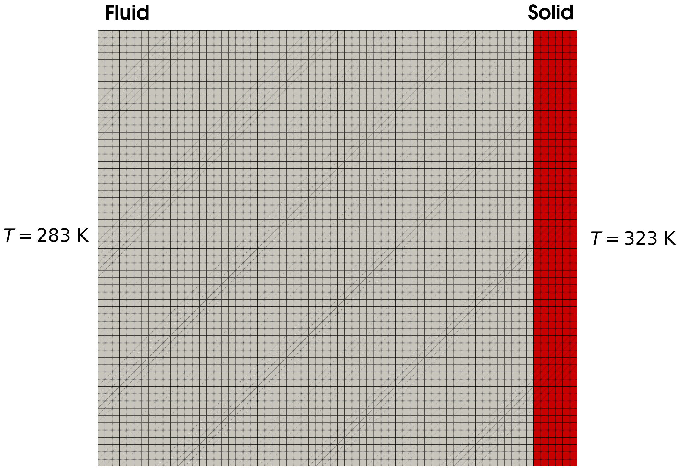
This case extends the traditional OpenFOAM cavity tutorial to include a coupled thermal analysis. The right wall of the cavity is assumed to be elastic and initially hotter than the cavity fluid (Figure 1). A coupled thermo-fluid-solid interaction analysis is performed where the heat equation is solved in the fluid and solid regions in addition to the Navier-Stokes equations in the fluid and the momentum equation in the solid. The coupling procedure enforces temperature and heat flux continuity at the fluid-solid interface. Within the fluid, the temperature differences generate forces that drive fluid flow, while in the solid, increases in temperature cause volumetric expansion.
At time \(t = 0\), the fluid temperature is \(283\) K, whereas the solid temperature is \(323\) K. The top, left, and bottom of the fluid domain are assumed to be stationary no-slip walls. The top and bottom of the solid domain are fixed (zero displacement), while the right has a zero-traction condition. The left of the fluid boundary is held at a fixed temperature of \(283\) K, while the right of the solid is held at \(323\) K. All other external boundaries are assumed to be adiabatic (zero heat flux). The right of the fluid domain and the left of the solid domain represent the fluid-solid interface, where kinematic (velocity continuity), kinetic (force continuity) and thermal constraints (temperature and heat flux continuity) are enforced. In both fluid and solid, gravity is assumed to act in the negative vertical direction \((0\;\)-\(9.81\; 0)\) m/s\(^{2}\) and inertial effects are included. Small deformations are assumed in the solid.
The end time is \(10\) s and time-step size \(\Delta t = 0.01\) s. The assumed fluid and solid physical parameters are given in Table 1. The solid behaviour is linear elastic, and plane strain conditions are assumed.
Table 1: Physical Parameters
| Parameter | Symbol | Value |
|---|---|---|
| Solid Young's Modulus | \(E\) | 1 kPa |
| Solid Density | \(\rho\) | 1 kg m\(^{-3}\) |
| Solid Poisson Ratio | \(\nu\) | 0.3 |
| Solid Coefficient of Thermal Expansion | \(\alpha\) | \(1\times10^{-5}\) K\(^{-1}\) |
| Solid Thermal Conductivity | \(k\) | \(0.04\) W/(m K) |
| Solid Specific Heat Capacity | \(C_p\) | \(1010\) J/(kg K) |
| Solid Reference Temperature | \(T_0\) | \(0\) K |
| Fluid Viscosity | \(\mu\) | 0.001 Pa s |
| Fluid Density | \(\rho\) | 1 kg m\(^{-3}\) |
| Fluid Coefficient of Thermal Expansion | \(\beta\) | \(2.85\times10^{-3}\) K\(^{-1}\) |
| Fluid Thermal Conductivity | \(\lambda\) | \(0.03\) W/(m K) |
| Fluid Specific Heat Capacity | \(C_p\) | \(1010\) J/(kg K) |
| Fluid Reference Temperature | \(T_{ref}\) | \(303\) K |
| Fluid Turbulent Prandtl Number | \(\text{Pr}_t\) | 0.85 |
| Gravity | \(g\) | \((0 \;\)-\(9.81 \; 0)\) m \(s^{-2}\) |
Results
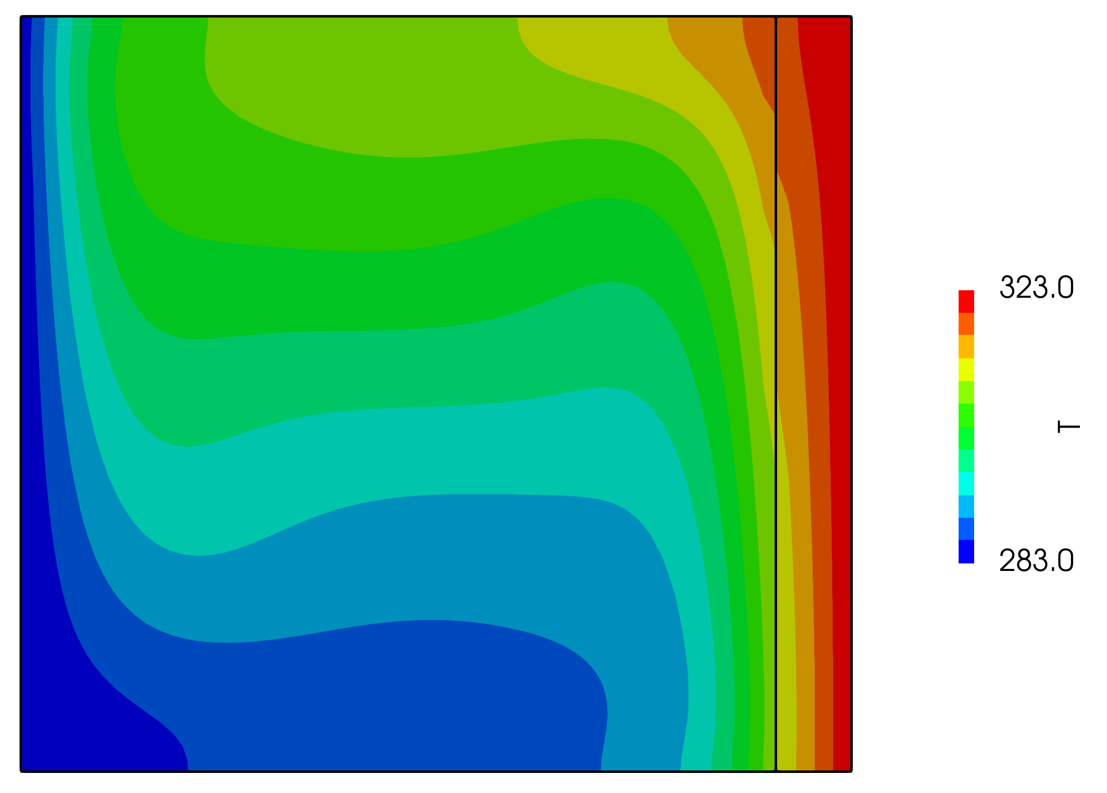
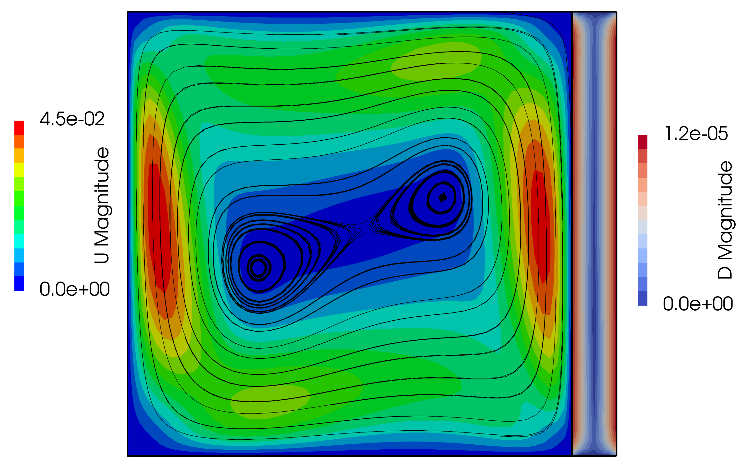
Over the duration of the simulation, the solid heats the fluid, causing a thermal circulation to form in the fluid. The evolution of the temperature of velocity fields is shown in Video 1. The temperature distribution at \(t = 10\) s is shown in Figure 2, and the fluid velocity and solid displacement fields are shown in Figure 3.
Video 1: Evolution of the temperature and velocity distributions within the fluid and solid domains
Running the Case
The tutorial case is located at solids4foam/tutorials/thermofluidSolidInteraction/thermalCavity. The case can be run using the included Allrun script, i.e. > ./Allrun. The Allrun script first executes blockMesh for both solid and fluid domains (> blockMesh -region fluid and > blockMesh -region solid ), and the solids4foam solver is used to run the case (> solids4Foam).