My fourth tutorial: 3dTube
Tutorial Aims
- Demonstrate the solution of an internal flow fluid-solid interaction problem;
- Demonstrate the fluid-solid interaction coupling approaches available in solids4foam;
- Provide insight into the relative performance of the different coupling approaches for internal flows;
- Examine the effect of time-step on the performance of the coupling approaches.
Case Overview
This case consists of a pressure pulse applied in a thick-walled elastic tube (Figure 1).
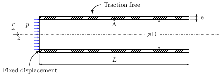
Figure 1: Wave propagation in an elastic pipe
The fluid is assumed incompressible, Newtonian and isothermal, with a density of 1000.0 kg/m3 and kinematic viscosity of 3e-6 m2/s. A pressure wave, with a peak of 1333.3 Pa, is applied at the tube inlet for a duration of 3e-3 s. The outlet pressure is held at 0 Pa throughout.
The tube wall is assumed an isotropic elastic body under the small-strain regime, modelled with Hooke's law, for consistency with the original publication that proposed this benchmark. The density is 1200.0 kg/m3, Young's modulus is 300 kPa, and Poisson's ratio is 0.3.
The case demonstrates a strong coupling between the fluid and the solid due to the high fluid-to-solid density ratio. When using a partitioned solution approach (as in solids4foam), the so-called ‘added-mass operator' makes the problem difficult to solve due to numerical instabilities.
Currently, in solids4foam, there are two classes of approaches for partitioned FSI coupling:
-
Dirichlet-Neumann coupling, where a Dirichlet condition is applied to the fluid velocity and Neumann conditions to the fluid pressure and solid displacement. This approach does not require modification of the underlying fluid solver; see Tuković Ž, Karač A, Cardiff P, Jasak H, Ivanković A, 2018, OpenFOAM finite volume solver for fluid–solid interaction. Trans FAMENA, 42(3):1–31.10.21278/TOF.42301;
-
Robin-Neumann coupling, where a Dirichlet condition is applied to the fluid velocity, a Robin condition to the fluid pressure, and a Neumann condition to the solid displacement. This approach does require modification of the underlying fluid solver, and hence it cannot be considered a black-box coupling approach; see Tuković Ž, Bukač M, Cardiff P, Jasak H, Ivanković A, 2018, Added mass partitioned fluid–structure interaction solver based on a robin boundary condition for pressure. In: OpenFOAM selected papers of the 11th workshop. Springer, Berlin, pp 1–23.
For each of these two classes of approach, we can employ different methods to accelerate the FSI iteration loop convergence; within solids4foam, we can use:
-
Aitken's dynamic relaxation;
-
the IQN-ILS algorithm of Joris Degroote, Robby Haelterman, Sebastiaan Annerel, Peter Bruggeman, Jan Vierendeels, Performance of partitioned procedures in fluid–structure interaction, Computers & Structures, 88, 7–8, 2010, 10.1016/j.compstruc.2009.12.006.
As well as using these acceleration algorithms, we can also use a weakly compressible fluid model rather than the standard fully incompressible model; for FSI, weakly compressible fluid models how been shown to improve convergence, for example, see E. Tandis and A. Ashrafizadeh, "A numerical study on the fluid compressibility effects in strongly coupled fluid–solid interaction problems," Engineering with Computers, 2019, doi: 10.1007/s00366-019-00880-4..
In this tutorial, we will compare six variants of the approaches above:
- Dirichlet-Neumann formulation with Aitken's acceleration and an incompressible fluid model: We use the
pimpleFluidfluid model. - Dirichlet-Neumann formulation with IQNILS acceleration and an incompressible fluid model: We use the
pimpleFluidfluid model. - Dirichlet-Neumann formulation with Aitken's acceleration and a weakly compressible fluid model: We use the
sonicLiquidFluidfluid model. - Dirichlet-Neumann formulation with IQNILS acceleration and a weakly compressible fluid model: We use the
sonicLiquidFluidfluid model. - Robin-Neumann formulation with an incompressible fluid: Support for this approach is implemented in the
pimpleFluidmodel, where we apply special interface boundary conditions:elasticWallPressurefor the fluid pressure field; andelasticWallVelocityfor the fluid velocity field. - Dirichlet-Neumann formulation with Aitken's acceleration and an incompressible fluid model using preCICE: This approach is the same as approach 1, except the preCICE coupling implementation is used. preCICE is an open-source coupling library for partitioned multi-physics simulations. In this case,
solids4Foamis used as the solid solver, and standardpimpleFoamis used as the fluid solver (as opposed to solids4foam'spimpleFluidfluid model). Due to implementation differences, this preCICE IQNILS approach may perform differently than the built-in solids4foam approach.
In all approaches, the solid domain setup is exactly the same, where an incremental small strain formulation is used (the linearGeometry solid model). One-quarter of the tube's cross-section is considered, although the case could actually be modelled as 2-D axisymmetric. The test is run for 0.02 s. A relatively tight FSI loop tolerance of 1e-6 is used for all approaches based on the interface motion. For approach 6 (preCICE), the relative displacement tolerance was set to 1e-6, and the relative force tolerance was set to 1e-3.
In all cases, the first-order Euler time scheme is used for the solid and fluid.
Running the Case
For approaches 1 to 4, the tutorial case is located at solids4foam/tutorials/fluidSolidInteraction/3dTube. The case can be run using the included Allrun scripts: Allrun.pimpleFluid for approaches 1 and 2, i.e../Allrun.pimpleFluid, and ./Allrun.sonicLiquidFluid for approaches 3 and 4. These scripts update the case with links to the correct files to be used by each approach. The acceleration algorithm, Aitken's or IQNILS, is specified in the constant/fsiProperties file.
For approach 5 (Robin-Neumann formulation), you should change the boundary conditions in the 0/fluid/p and 0/fluid/U files to the elastic* versions; currently, the Robin approach is only available in foam-extend-4.1.
The tutorial case for approach 6, which uses preCICE, is located at solids4foam/tutorials/fluidSolidInteraction-preCICE/3dTube; once again, the Allrun script runs the case.
Remember that a tutorial case can be cleaned and reset using the included Allrun script, i.e. ./Allclean.
Expected Results
This case has been proposed as a benchmark for FSI problems. The solution for point A's (see Figure 1) axial and radial displacement is available in: A. Lozovskiy, M. A. Olshanskii, and Y. V. Vassilevski, "Analysis and assessment of a monolithic FSI finite element method," Computers and Fluids, vol. 179, pp. 277–288, 2019, doi: 10.1016/j.compfluid.2018.11.004.
Large Time Step
Initially, we compare the solutions using a relatively large time step size of 1e-4 s. Figure 2 shows the radial displacement at point A vs time, Figure 3 shows the axial displacement at point A vs time, and Figure 4 shows the iterations per time step. In the figures, the approaches are designated as:
- DNF-Aitken: Dirichlet-Neumann formulation with Aitken's acceleration and an incompressible fluid model;
- DNF-IQNILS: Dirichlet-Neumann formulation with IQNILS acceleration and an incompressible fluid model;
- WC-DNF-Aitken: Dirichlet-Neumann formulation with Aitken's acceleration and a weakly compressible fluid model;
- WC-DNF-IQNILS: Dirichlet-Neumann formulation with IQNILS acceleration and a weakly compressible fluid model;
- RNF: Robin-Neumann formulation with an incompressible fluid;
- preCICE-DN-IQNILS: Dirichlet-Neumann formulation with Aitken's acceleration and an incompressible fluid model using preCICE.
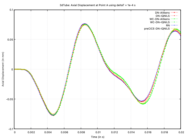
Figure 2: Axial displacement at point A vs time with deltaT = 1e-4 s
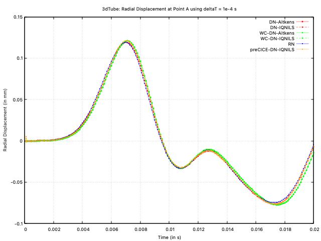
Figure 3: Radial displacement at point A vs time with deltaT = 1e-4 s
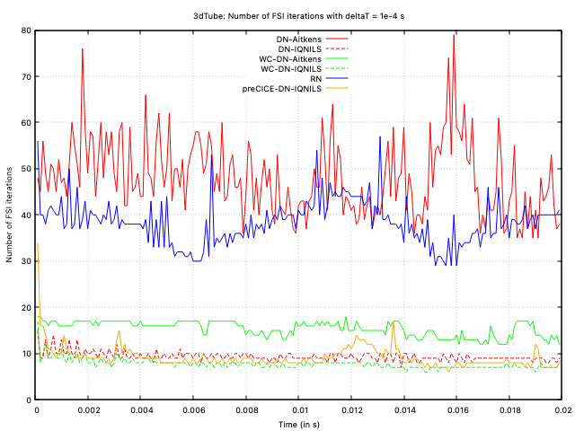
Figure 4: Number of FSI iterations per time-step with deltaT = 1e-4 s
The predictions from all approaches agree closely. Examining the number of FSI iterations per time step, both implementations (solids4foam and preCICE) of Dirichlet-Neumann coupling with IQN-ILS acceleration are seen to require the least number of iterations. The weakly compressible approach is the next best performing approach, while the incompressible Aitken's-accelerated Dirichlet-Neumann and Robin-Neumann approaches are seen to perform the poorest.
Small Time Step
To observe the effect of the time step size, the cases were re-run with a smaller time step of 2.5e-5 s, where Figures 5, 6 and 7 show the radial displacement, axial displacement and the number of iterations. 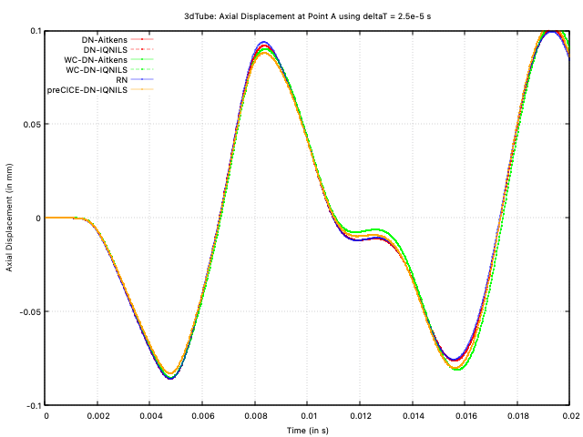
Figure 5: Axial displacement at point A vs time with deltaT = 2.5e-5 s
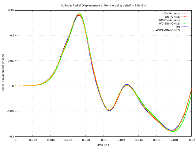
Figure 6: Radial displacement at point A vs time with deltaT = 2.5e-5 s
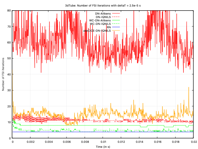
Figure 7: Number of FSI iterations per time-step with deltaT = 2.5e-5 s
Unlike the larger time step, the Robin-Neumann approach now requires the least number of iterations per time step (exactly 4 for every time step). The weakly compressible approaches are the next best, where the IQNILS-accelerated compressible model outperforms the Aitken's-accelerated compressible model. The incompressible IQNILS approaches are the next best (both solids4foam and preCICE). Finally, in this case, the Aitken's-accelerated incompressible model shows the poorest performance, requiring an order of magnitude greater number of iterations than the best approach. The impressive performance of the Robin-Neumann approach can also be observed for smaller time steps; in general, for cases like this, if the time step is sufficiently small, the Robin-Neumann approach requires minimal iterations; however, once the time step is large, then the Robin approach diverges or becomes uncompetitive.
First-Order Euler vs Second-Order Backward Time Schemes
Finally, we demonstrate the effect of the time scheme by comparing the first-order Euler and second-order backward time schemes, where both the solid and fluid use the same time schemes. For this, we re-run the case with five time step sizes: 8e-4, 4e-4, 2e-4, 1e-4 and 5e-5 s. Figure 8 shows the first-order Euler radial displacements results, Figure 9 shows the second-order backward results, and Figure 10 compares both. The second-order scheme shows small time discretisation errors for each time step and is seen to converge more quickly as the time step size is reduced, as expected. The results were generated using the weakly compressible fluid model and Aitken's coupling; however, the same behaviour is expected with the other modelling and coupling approaches.
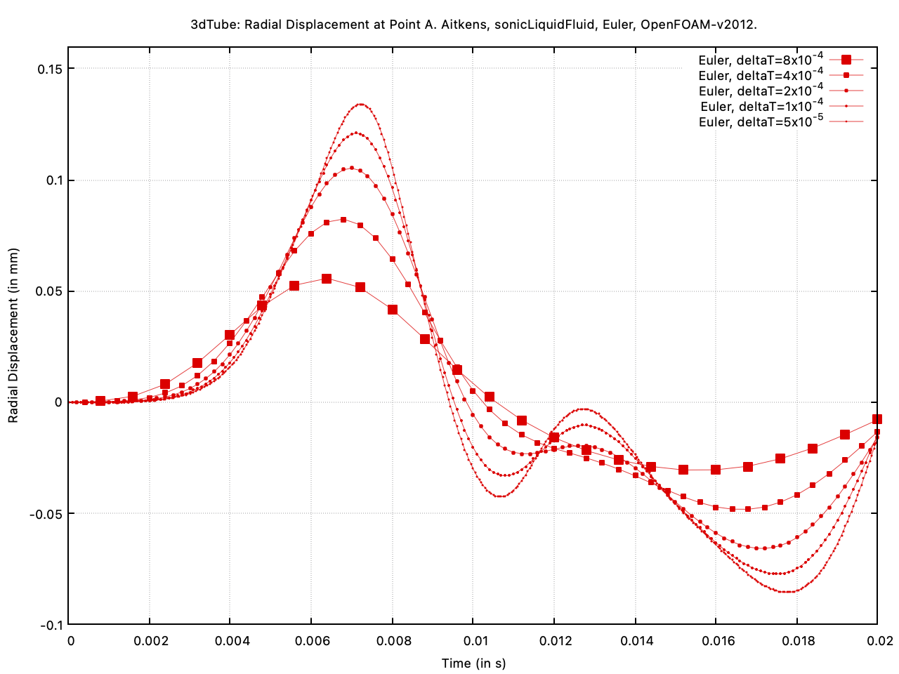
Figure 8: The effect of the time step size when using the first-order Euler time scheme
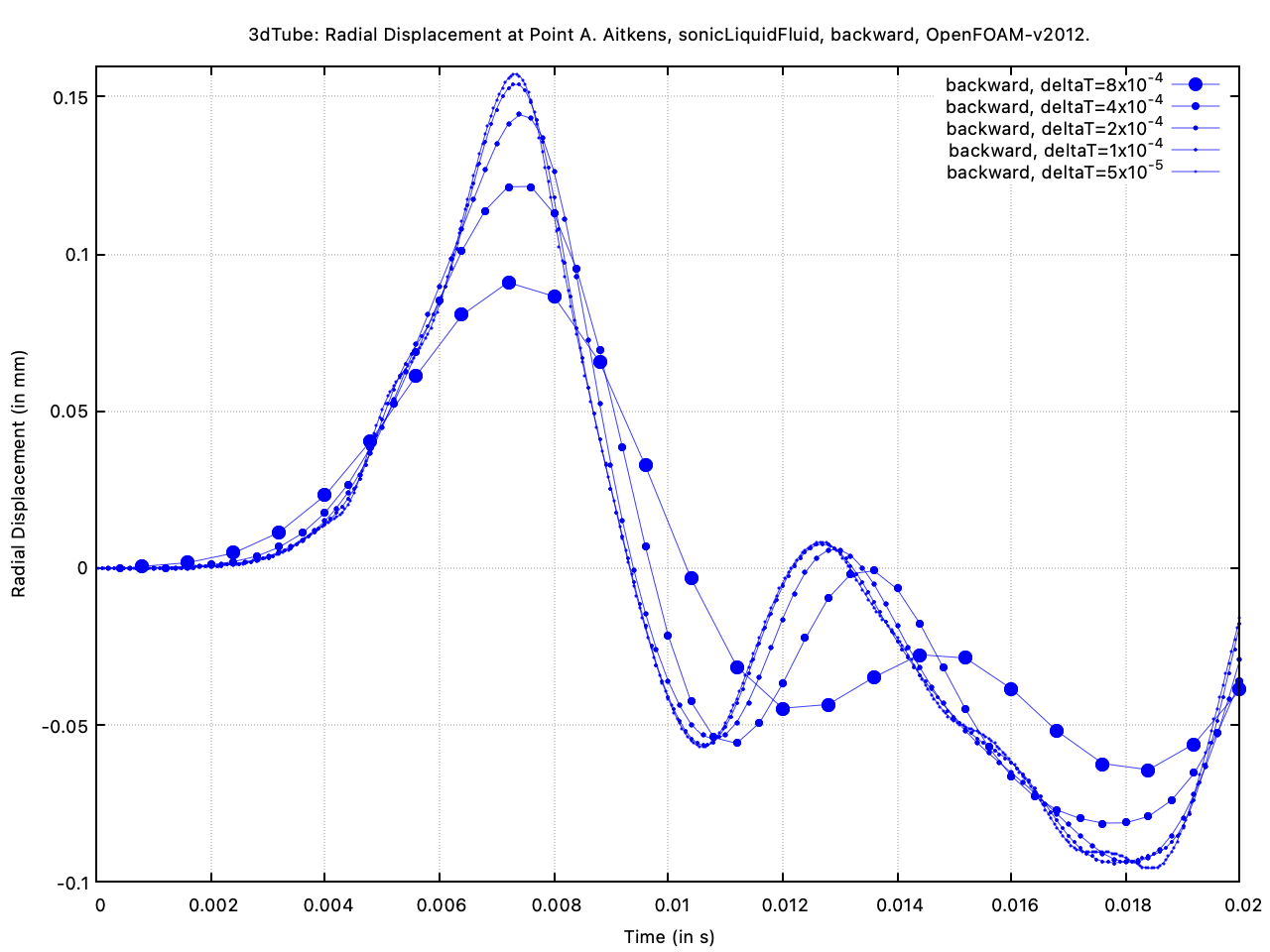
Figure 9: The effect of the time step size when using the second-order backward time scheme
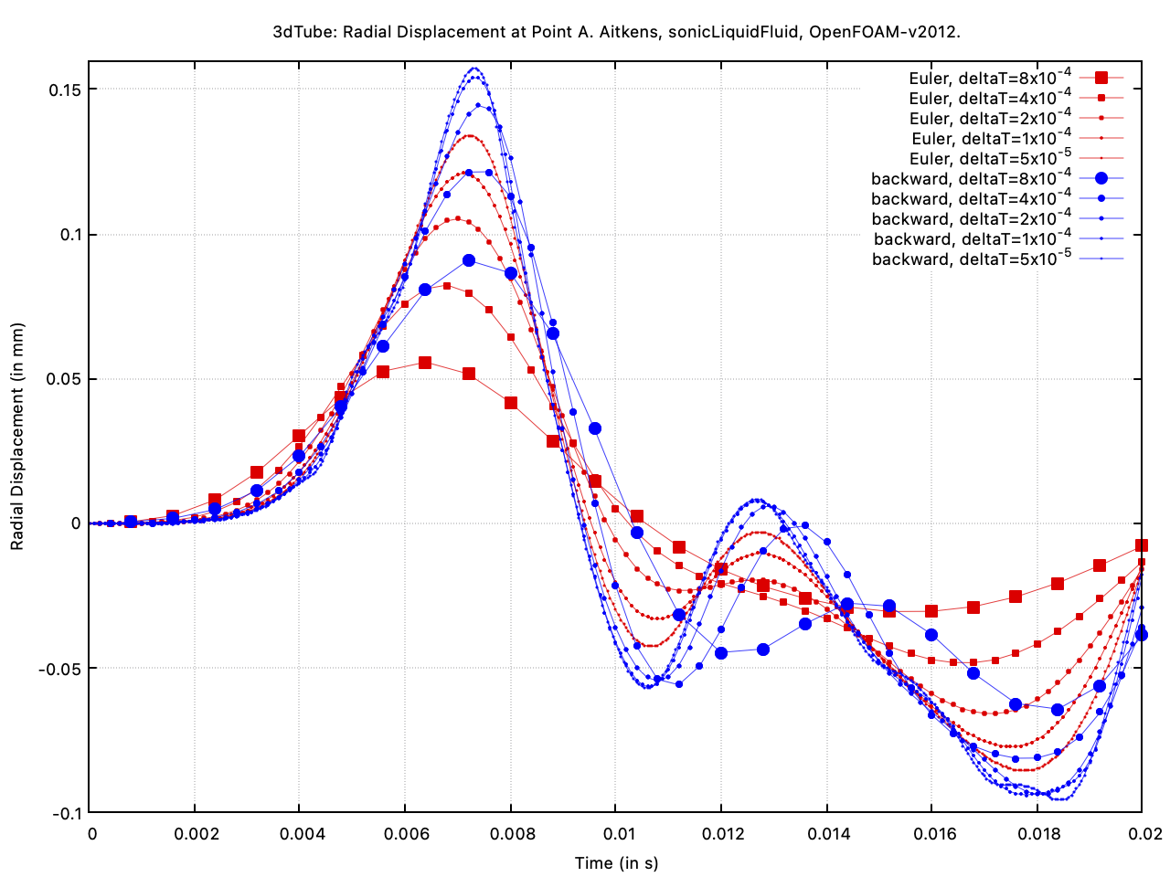
Figure 10: Comparing the first-order Euler and second-order backward schemes as the time step size is reduced
Table 1 gives the total clock time for each model when running these models in serial. Surprisingly, the fastest model is the backward method with the smallest time step (5e-5 s). The fastest Euler model uses the largest time step (8e-4 s), but next fastest model uses the second smallest time step (1e-4 s). The explanation for this is that when using larger time steps, a much greater number of outer fluid-solid interaction iterations are required; whereas for smaller time steps, much fewer iterations are required, possibly resulting in a lower overall clock time. If the time step sizes were reduced further, it would be expected that at some point, the models would start to become slower (e.g., as shown by the Euler method when going from 1e-4 to 5e-5 s); however, these results highlight the importance of selecting a sufficiently small time step size for fluid-solid interaction simulations.
| Time Step Size (in s) | Euler (in s) | backward (in s) |
|---|---|---|
| 8e-4 | 1568 | 2233 |
| 4e-4 | 2618 | 2710 |
| 2e-4 | 3009 | 2451 |
| 1e-4 | 2021 | 1999 |
| 5e-5 | 2718 | 1648 |
Table 1: Clock times for the Euler and backward with different time step sizes
Data Availability
The results and gnuplot scripts used to generate the figures above are available in the solids4foam tutorials benchmark data repository.