Thermally loaded cylinder: `hotCylinder`

Prepared by Philip Cardiff and Ivan Batistić

Tutorial Aims

Demonstrate the solution of a thermo-elastic problem;
Compare the solver accuracy for a thermo-elastic problem against the available analytical solution.

Case Overview

This case considers a thick-walled cylinder subjected to a temperature difference between the inner (\(r_i=0.5\) m) and outer (\(r_o=0.7\) m) surfaces. The problem is considered plane strain, with a quarter of the domain modelled because of symmetry. Gravity is neglected, and the case is simulated as a steady state using one loading step. The outside and inner cylinder surfaces are modelled as stress-free. The inner cylinder surface has a prescribed temperature of \(T_i=100\) K and the outer of \(T_o=0\) K. The cylinder material has a Poisson's ratio of \(\nu=0.3\), a Young's modulus of \(E = 200\) GPa and a coefficient of linear thermal expansion of \(\alpha = 1\times 10^{-5}\) K\(^{-1}\). The cylinder is discretised with \(10\) cells in the radial direction and \(60\) cells in the circumferential direction.

Expected Results

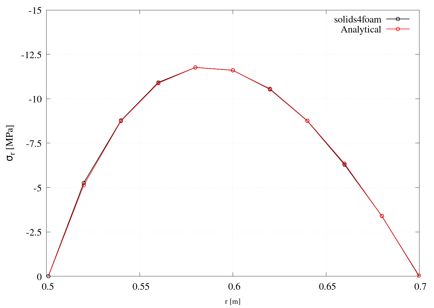
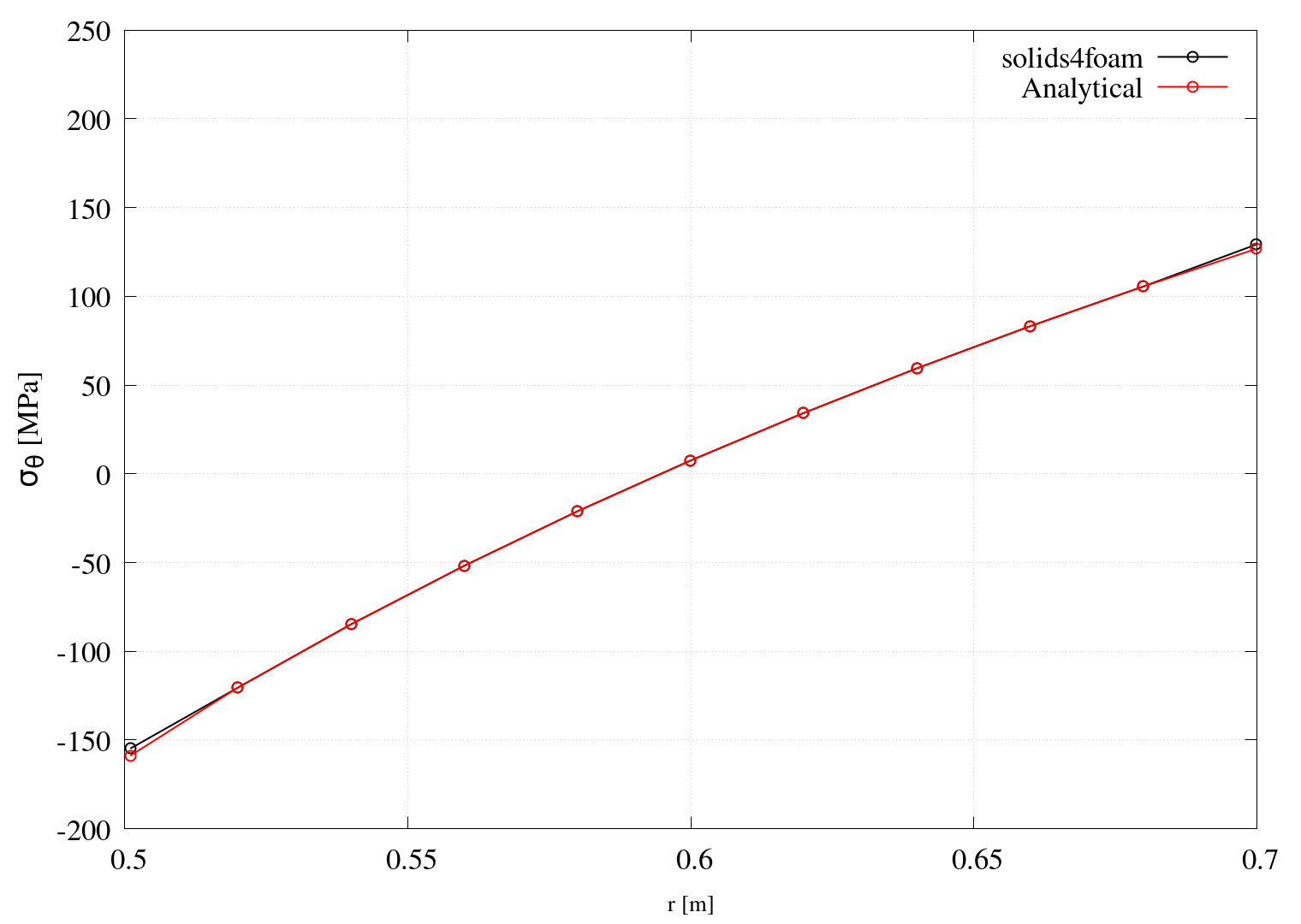
Comparison between numerical and analytical solutions is performed in terms of circumferential and radial stresses in the radial direction through the cylinder, for which the analytical solutions are as follows [1]:

\[\sigma_r = \dfrac{\alpha E (T_i-T_o)}{2(1-\nu)\ln\dfrac{r_o}{r_i}}\left[-\ln\dfrac{r_o}{r}-\dfrac{r_i^2}{r_o^2-r_i^2}\left(1-\dfrac{r_o^2}{r^2}\right) \ln\dfrac{r_o}{r_i} \right],\] \[\sigma_{\theta} = \dfrac{\alpha E (T_i-T_o)}{2(1-\nu)\ln\dfrac{r_o}{r_i}}\left[1-\ln\dfrac{r_o}{r}-\dfrac{r_i^2}{r_o^2-r_i^2}\left(1+\dfrac{r_o^2}{r^2}\right) \ln\dfrac{r_o}{r_i} \right],\] \[\sigma_z = \dfrac{\alpha E (T_i-T_o)}{2(1-\nu)\ln\dfrac{r_o}{r_i}}\left[1-2\ln\dfrac{r_o}{r}-\dfrac{2r_i^2}{r_o^2-r_i^2} \ln\dfrac{r_o}{r_i} \right].\]

The analytical equation for temperature distribution is [1]:

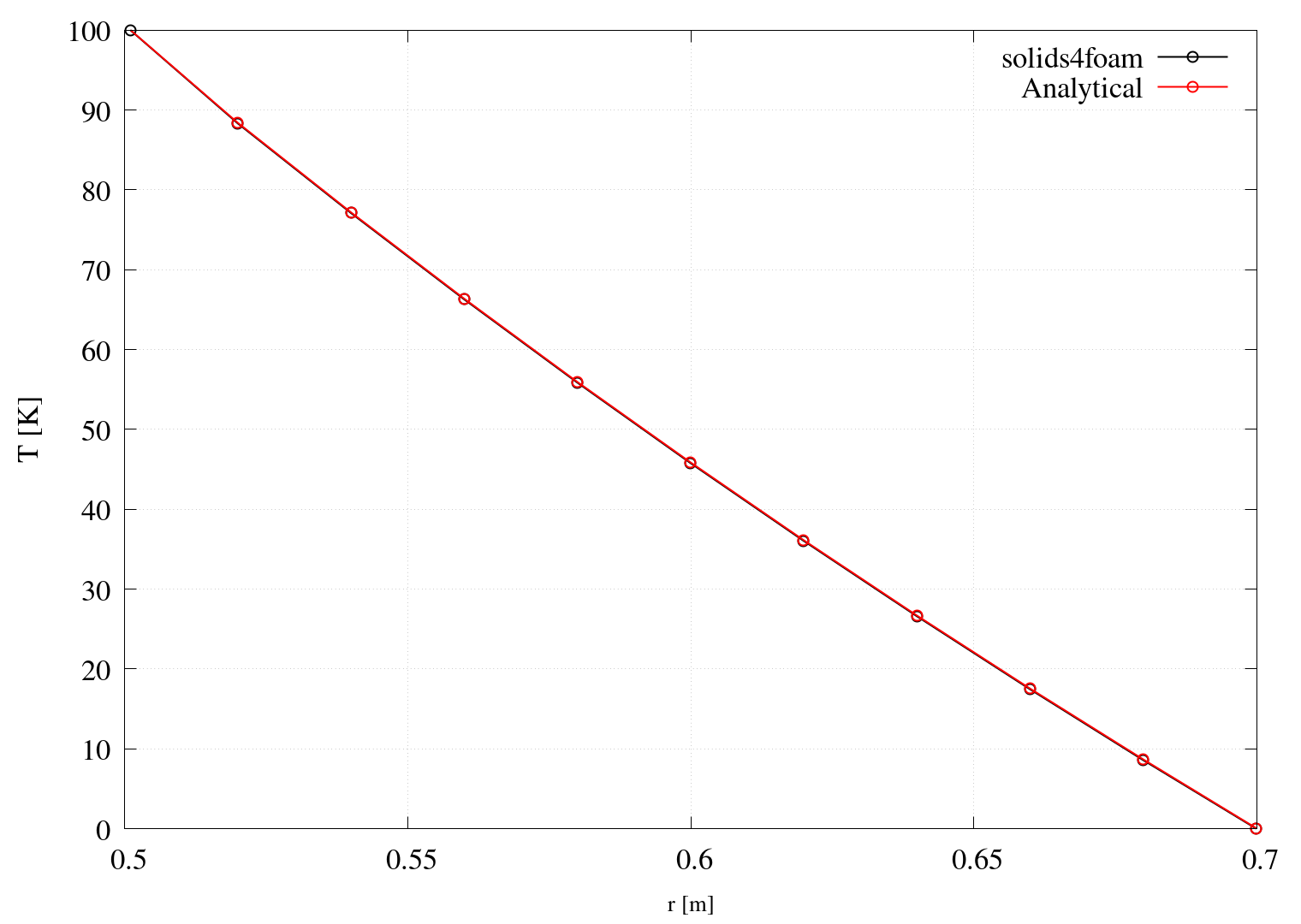
\[T = \dfrac{(T_i - T_o)}{\ln\dfrac{r_o}{r_i}}\ln\dfrac{r_o}{r}.\]

The hotCylinderAnalyticalSolution function object in system/controlDict is used to generate analytical solution fields (analyticalT, analyticalRadialStress and analyticalHoopStress):

analyticalHotCylinder
{
	type    hotCylinderAnalyticalSolution;

    // Inner pipe radius
    rInner  0.5;

    // Outer pipe radius
    rOuter  0.7;

	// Inner pipe temperature
    TInner  100;

    // Outer pipe temperature
    TOuter  0;

    // Young's modulus
    E       200e9;

    // Poisson's ratio
    nu      0.3;

    // Coefficient for linear thermal expansion
    alpha   1e-5;
}

  

Note

hotCylinderAnalyticalSolution function object does not read mechanicalProperties dictionary; therefore, it requires entering all material data that should correspond to those used in the case.

The transformStressToCylindrical function object in system/controlDict is used to transform the \(\sigma\) stress tensor from Cartesian coordinates to the cylindrical:

transformStressToCylindrical
{
    type        transformStressToCylindrical;
    origin      (0 0 0);
    axis        (0 0 1);
}
  

Analytical solution fields generated by the hotCylinderAnalyticalSolution function object, the cylindrical stresses (sigma:Transformed) and the temperature field T are plotted along a \(\theta=45^{\circ}\) line using the sample utility:

fields( sigma:Transformed analyticalRadialStress analyticalHoopStress T analyticalT );

sets
(
    line
    {
        type       face;
        axis       distance;
        start      (0.0 0.0 0.05);
        end        (0.5 0.5 0.05);
    }
);
  

If gnuplot is installed, Figures 1, 2 and 3 are automatically generated when running the case using the Allrun script. Figures 1 and 2 compare the analytical solutions with the numerically calculated ones.

Figure 1: Radial stress

Figure 2: Circumferential stress

Figure 3: Temperature profile

Running the Case

The tutorial case is located at solids4foam/tutorials/solids/thermoelasticity/hotCylinder/hotCylinder. The case can be run using the included Allrun script, i.e. > ./Allrun. In this case, the Allrun creates the mesh using blockMesh (> blockMesh), followed by running the case with the solids4Foam solver (> solids4Foam). As the last step, the sample utility is used to extract data along \(\theta=45^{\circ}\) line. Optionally, if gnuplot is installed, the temperature profile and the profile of the radial and circumferential stresses are plotted in the T.png, sigmaR.png and sigmaTheta.png files.

References

[1] S. Timoshenko and J. Goodier, Theory of Elasticity. McGraw-Hill, 3 ed., 1970.

Thermally loaded cylinder: hotCylinder