My first tutorial: hotSphere
Tutorial Aims
- Demonstrate how to perform a solid-only analysis in solids4foam;
- Describe the structure of a solids4foam solid-only case;
- Demonstrate how to perform a thermo-elastic analysis;
Case Overview
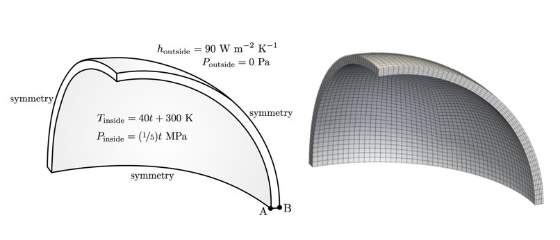
This case analyses the stresses and displacements generated in a spherical pressure vessel subjected to an increasing internal pressure and temperature. The problem is 1-D axisymmetric in nature, but for demonstration purposes one eighth of the vessel is modelled here and symmetry planes are used. The outer surface of the vessel is stress/traction free and the heat flux is given by Newton's law of cooling (a simplified convection boundary condition). The internal pressure and temperature are a function of time $t$: \(\begin{align} T_{\text{inside}} = 40t + 300 ~\text{K} \\ p_{\text{inside}} = (1/5)t ~\text{MPa} \end{align}\)
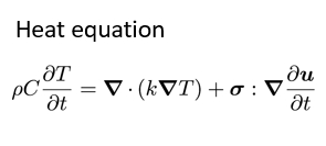
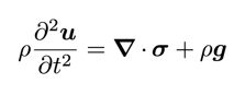
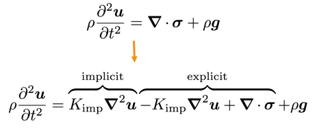
We expect the vessel to deform due to the applied pressure and also due to the thermal gradient. The deformations (strains/rotations) are expected to be "small": this means we can use a small strain (linear geometry) approach, where the displacements are assumed not to affect the material geometry. The governing equations are given by the conservation equations are linear momentum (linear geometry form) and energy (heat equation form): 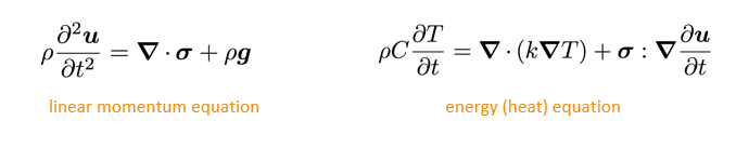
In this case, the solver employs a segregated solution methodology, where a loop is performed over the momentum equation (solved for displacement D) and the energy equation (solved for temperature T) until convergence is achieved. This loop is performed within each time-step resulting in an overall method that is implicit in time.
for all time-steps
    do
        solve energy equation for T (terms depending on D are calculated explicitly)
        solve momentum equation for D (terms depending on T are calculated explicitly)
    while not converged
end
Expected Results
At 5 s, the expected temperature distribution across the wall thickness is expected to be close to linear, where, the von Mises stress distribution is quite nonlinear with a minimum 4 mm from the inner wall. 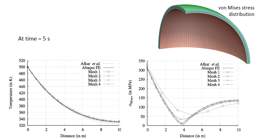
Running the Case
As in all solids4foam tutorials, the tutorial case can be run using the included Allrun script, i.e. > ./Allrun. In this case, the Allrun script is
#!/bin/bash

# Source tutorial run functions
. $WM_PROJECT_DIR/bin/tools/RunFunctions

# Source solids4Foam scripts
source solids4FoamScripts.sh

# Check case version is correct
solids4Foam::convertCaseFormat .

# Create the mesh
solids4Foam::runApplication fluentMeshToFoam hotSphere.msh

# Run the solver
solids4Foam::runApplication solids4Foam
where the solids4Foam::convertCaseFormat . script makes minor changes to the case to make it compatible with your version of OpenFOAM/foam-extend. As can be seen, the mesh in the fluent format is converted to the OpenFOAM format before running the solids4Foam solver.
A tutorial case can be cleaned and reset using the included Allrun script, i.e. > ./Allclean.
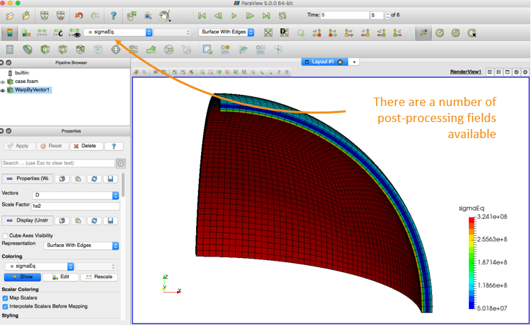
Analysing the Results
When viewing the results in ParaView, it can be insightful to warp the geometry by a scaled displacement field. This can be achieved using the Warp By Vector filter, where the D displacement field is selected as the Vector and a Scale Factor of 1 shows the true deformation. In this case, using a Scale Factor of 100 allows the deformation to be seen. 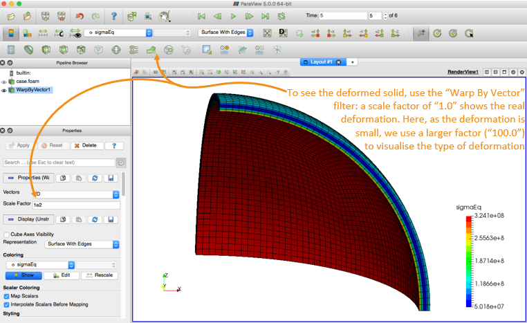
Delving Deeper
If you would like to learn more about the case, then please continue; if not, how about you check out another tutorial.
Case Structure
The case structure follows the typical OpenFOAM case structure:
hotSphere
├── 0
│   ├── D
│   └── T
├── Allclean
├── Allrun
├── constant
│   ├── dynamicMeshDict
│   ├── g
│   ├── mechanicalProperties
│   ├── physicsProperties
│   ├── polyMesh
│   │   └── …
│   ├── solidProperties
│   ├── thermalProperties
│   ├── timeVsPressure
│   └── timeVsTemperature
├── hotSphere.msh
└── system
    ├── controlDict
    ├── fvSchemes
    └── fvSolution
Initial Conditions and Boundary Conditions
In this case, there are two primitive variables:
- displacement (vector)
- temperature (scalar)
├── 0
│   ├── D   displacement vector field
│   └── T   temperature scalar field
This initial displacement field is assumed to be zero, and the initial temperature field is assumed to be 300 K.
Displacement Field D Boundary Conditions
A zero-traction condition is specified on the outer wall:
outside
{
    type            solidTraction;
    traction        uniform ( 0 0 0 );
    pressure        uniform 0;
    value           uniform (0 0 0);
}
pressure here is referring to the normal component of the boundary traction vector; in general, this is not the same as the hydrostatic pressure. The total applied traction is: appliedTraction = traction - n*pressure where n is the boundary unit normal field.
A time-varying traction condition is given on the inner wall:
inside
{
    type            solidTraction;
    traction        uniform ( 0 0 0 );
    pressureSeries
    {
        "file|fileName" "$FOAM_CASE/constant/timeVsPressure";
        outOfBounds clamp;
    }
    value           uniform (0 0 0);
}
where timeVsPressure specifies time vs pressure as a XY piecewise linear series:
(
    ( 0 0 )
    ( 5 1e6 )
)
Temperature Field T Boundary Conditions
For the temperature field, a convection condition (Newton's law of cooling) is specified on the outer wall:
outside
{
    type            thermalConvection;
    alpha           uniform 90;
    Tinf            300;
    value           uniform 300;
}
A time-varying temperature is given on the inside wall:
inside
{
    type            fixedTemperature;
    temperatureSeries
    {
       fileName "$FOAM_CASE/constant/timeVsTemperature";
       outOfBounds clamp;
    }
    value           uniform 300;
}
where timeVsTemperature specifies time vs temperature:
(
    ( 0 300 )
    ( 5 500 )
)
Specifying the Type of Solid Analysis
The type of solid analysis, which is called by the solids4Foam solver, is specified in the constant/solidProperties dictionary:
solidModel thermalLinearGeometry;

thermalLinearGeometryCoeffs
{
    nCorrectors          10000;

    solutionTolerance    1e-6;

    alternativeTolerance 1e-7;

    infoFrequency        100;
}
Here, the thermalLinearGeometry is a solid mathematical model where the heat equation is solved (thermal-) and a linear geometry (-LinearGeometry) mechanical approach is taken.
A linear geometry approach is also known as a “small strain” or “small strain/rotation” approach and means that we assume the cell geometry (volumes, face areas, etc.) to be independent of the displacement field. This assumption is typically OK when the deformation is “small”.
nCorrectors: this is the maximum number of outer correctors per time-step. IfnCorrectorsis reached, this means the equations have not converged to the required tolerance.solutionToleranceandalternativeTolerance: these are solution tolerances for the outer corrector loop. Further details are given below.- Iterations will continue until either the D (and T) have converged to the specific tolerances or the maximum number of correctors has been reached.
infoFrequency: this is the frequency that the outer loop residuals are printed to the standard output.
The Mechanical Law
A "solid" analysis requires the definition of the mechanical properties via the mechanicalProperties dictionary; in this case the thermoLinearElastic law is specified (Duhamel-Nuemann form of Hooke's law): 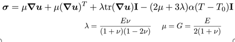
mechanical
(
    steel
    {
        type  thermoLinearElastic;
        rho   rho [1 -3 0 0 0 0 0] 7750;
        E     E [1 -1 -2 0 0 0 0] 190e+9;
        nu    nu [0 0 0 0 0 0 0] 0.305;
        alpha alpha [0 0 0 -1 0 0 0] 9.7e-06;
        T0    T0 [0 0 0 1 0 0 0] 300;
    }
);
where, in addition to the density, three mechanical properties must be specified: Elastic/Young's modulus E, Poisson's ratio ν and the coefficient of linear thermal expansion α.
As we are performing a heat analysis, so we also need to specify the thermal properties via the thermalProperties dictionary. In this case the constant law is specified (Fourier's conduction law) by specific heat C and thermal conductivity k: 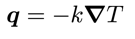
thermal
{
    type      constant;
    C         C [0 2 -2 -1 0 0 0] 486;
    k         k [1 1 -3 -1 0 0 0] 20;
}
Examining the Solver Output
Let us examine the output from the solids4Foam solver for this case:
Time = 1

Evolving thermal solid solver
Solving coupled energy and displacements equation for T and D
    Corr, res (T & D), relRes (T & D), matRes, iters (T & D)
    100, 3.37856e-10, 9.48897e-06, 0, 3.1907e-05, 0, 0, 12
    200, 1.97288e-10, 2.07022e-06, 0, 7.17093e-06, 0, 0, 10
    300, 9.26738e-10, 4.86841e-07, 0, 1.6726e-06, 0, 0, 10
    The residuals have converged
    337, 1.64639e-10, 2.83573e-07, 0, 9.86025e-07, 0, 0, 12

Max T = 340
Min T = 301.118
Max magnitude of heat flux = 321505
Max epsilonEq = 0.000254994
Max sigmaEq (von Mises stress) = 5.56883e+07
ExecutionTime = 8.73 s  ClockTime = 9 s
For solid analyses, the solids4Foam solver checks three types of residuals:
res: linear solver residualrelRes: relative residual - change of the primitive variablematRes: material residual - for nonlinear material laws
where the tolerances are specified in the solidProperties dictionary. In this case, there are residuals for T and D. The material residual is zero because a linear mechanical law was selected (no need to iterate).
fvSchemes
Switching between steadyState and transient analyses requires changing the d2dt2 and ddt schemes.
The gradient schemes should almost always be leastSquares as the standard Gauss linear method can produce large errors in the stress field for skewed cells, e.g. on the plateHole case 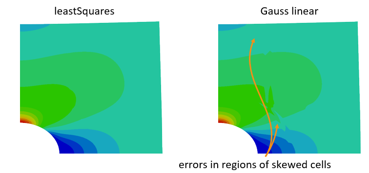
fvSolution
The D and T equations are similar to the p equation in standard CFD approaches; as such, the preconditioned conjugate gradient (PCG) or the algebraic multi-grid (GAMG) linear solvers tend to work best. The relTol can set be 0.1 as outer iterations are performed over the momentum equation until convergence.
In general, the D equation and D field do not require under-relaxation; however, it is beneficial or required in some cases:
- equation relaxation
- to restrict rigid body motion in contact analysis
- field relaxation
- complex boundary conditions
- complex material behaviour, e.g. plasticity
- large strains
- poor meshes
Equation relaxation values of 0.99-0.9999 are typical, while field relaxation factors should typically be greater than 0.1.
Code
solidModel
For the hotSphere test case, we have selected a "solid" analysis in the physicsProperties dictionary: this means a solidModel class will be selected; then, we specify the actual solidModel class to be the thermoLinGeomSolidModel class.
The code for the thermoLinGeomSolidModel class is located at:
solids4foam/src/solids4FoamModels/solidModels/thermalLinGeomSolid/thermalLinGeomSolid.C
Let us examine the "evolve" function of this class to see the equations solved:
bool thermalLinGeomSolid::evolve()
{
    Info<< "Evolving thermal solid solver" << endl;

    int iCorr = 0;
    lduSolverPerformance solverPerfD;
    lduSolverPerformance solverPerfT;
    blockLduMatrix::debug = 0;

    Info<< "Solving coupled energy and displacements equation for T and D"
        << endl;

    // Momentum-energy coupling outer loop
    do
    {
        // Store fields for under-relaxation and residual calculation
        T().storePrevIter();

        // Heat equation
        fvScalarMatrix TEqn
        (
            rhoC_*fvm::ddt(T_)
         == fvm::laplacian(k_, T_, "laplacian(k,T)")
          + (sigma() && fvc::grad(U()))
        );
...
        // Under-relaxation the linear system
        TEqn.relax();

        // Solve the linear system
        solverPerfT = TEqn.solve();

        // Under-relax the field
        T_.relax();

        // Update gradient of temperature
        gradT_ = fvc::grad(T_);

        // Store fields for under-relaxation and residual calculation
        D().storePrevIter();

        // Linear momentum equation total displacement form
        fvVectorMatrix DEqn
        (
            rho()*fvm::d2dt2(D())
         == fvm::laplacian(impKf_, D(), "laplacian(DD,D)")
          - fvc::laplacian(impKf_, D(), "laplacian(DD,D)")
          + fvc::div(sigma(), "div(sigma)")
          + rho()*g()
          + mechanical().RhieChowCorrection(D(), gradD())
        );
...
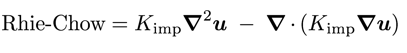
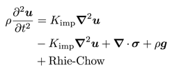
Also, we add an additional diffusion term to quell numerical oscillations (e.g. checker-boarding) based on Rhie-Chow correction:
        // Under-relaxation the linear system
        TEqn.relax();

        // Solve the linear system
        solverPerfT = TEqn.solve();

        // Under-relax the field
        T_.relax();

        // Update gradient of temperature
        gradT_ = fvc::grad(T_);

        // Store fields for under-relaxation and residual calculation
        D().storePrevIter();

        // Linear momentum equation total displacement form
        fvVectorMatrix DEqn
        (
            rho()*fvm::d2dt2(D())
         == fvm::laplacian(impKf_, D(), "laplacian(DD,D)")
          - fvc::laplacian(impKf_, D(), "laplacian(DD,D)")
          + fvc::div(sigma(), "div(sigma)")
          + rho()*g()
          + mechanical().RhieChowCorrection(D(), gradD())
        );
...
        // Under-relaxation the linear system
        DEqn.relax();

        // Solve the linear system
        solverPerfD = DEqn.solve();

        // Under-relax the field
        relaxField(D(), iCorr);

        // Update increment of displacement
        DD() = D() - D().oldTime();

        // Update velocity
        U() = fvc::ddt(D());

        // Update gradient of displacement
        mechanical().grad(D(), gradD());

        // Update gradient of displacement increment
        gradDD() = gradD() - gradD().oldTime();

        // Calculate the stress using run-time selectable mechanical law
        mechanical().correct(sigma());
    }
    while
    (
        !converged(iCorr, solverPerfD, solverPerfT, D(), T_)
     && ++iCorr < nCorr()
    ); // loop around TEqn and DEqn

    // Interpolate cell displacements to vertices
    mechanical().interpolate(D(), pointD());

    // Increment of displacement
    DD() = D() - D().oldTime();

    // Increment of point displacement
    pointDD() = pointD() - pointD().oldTime();

    return true;
}
The values of impK can affect convergence, but not the answer, assuming convergence is achieved.
mechanicalLaw
For the hotSphere test case, we have selected the thermoLinearElastic mechanical law in the mechanicalProperties dictionary: this class will perform the calculation of stress for the solid.
The code for the thermoLinearElastic mechanical law class is located at:
solids4foam/src/solids4FoamModels/materialModels/mechanicalModel/mechanicalLaws/linearGeometryLaws/thermoLinearElastic/thermoLinearElastic.C
which calculates the stress according to the Duhamel-Neumann form of Hooke's law: 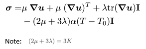
Let us examine the "correct" function of this class to see how the stress is calculated:
void Foam::thermoLinearElastic::correct(volSymmTensorField& sigma)
{
    // Calculate linear elastic stress
    linearElastic::correct(sigma);

    if (TPtr_.valid())
    {
        // Add thermal stress component
        sigma -= 3.0*K()*alpha_*(TPtr_() - T0_)*symmTensor(I);
    }
    else
    {
        // Lookup the temperature field from the solver
        const volScalarField& T = mesh().lookupObject<volScalarField>("T");

        // Add thermal stress component
        sigma -= 3.0*K()*alpha_*(T - T0_)*symmTensor(I);
    }
}
As thermoLinearElastic derives from the linearElastic law, we will also examine the "correct" function for this class:
solids4foam/src/solids4FoamModels/materialModels/mechanicalModel/mechanicalLaws/linearGeometryLaws/linearElastic/linearElastic.C
void Foam::linearElastic::correct(volSymmTensorField& sigma)
{
// Calculate total strain
if (incremental())
{
// Lookup gradient of displacement increment
const volTensorField& gradDD =
mesh().lookupObject<volTensorField>("grad(DD)");
epsilon_ = epsilon_.oldTime() + symm(gradDD);
}
else
{
// Lookup gradient of displacement
const volTensorField& gradD =
mesh().lookupObject<volTensorField>("grad(D)");
epsilon_ = symm(gradD);
}
// For planeStress, correct strain in the out of plane direction
if (planeStress())
{
if (mesh().solutionD()[vector::Z] > -1)
{
FatalErrorIn
(
"void Foam::linearElasticMisesPlastic::"
"correct(volSymmTensorField& sigma)"
) << "For planeStress, this material law assumes the empty "
<< "direction is the Z direction!" << abort(FatalError);
}
epsilon_.replace
(
symmTensor::ZZ,
-(nu_/E_)
*(sigma.component(symmTensor::XX) + sigma.component(symmTensor::YY))
);
}
// Hooke's law : standard form
//sigma = 2.0*mu_*epsilon_ + lambda_*tr(epsilon_)*I + sigma0_;
// Hooke's law : partitioned deviatoric and dilation form
const volScalarField trEpsilon = tr(epsilon_);
calculateHydrostaticStress(sigmaHyd_, trEpsilon);
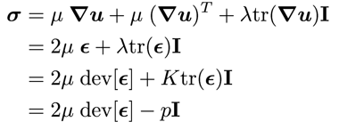
sigma = 2.0*mu_*dev(epsilon_) + sigmaHyd_*I + sigma0_;
}
where sigma0_ is an optional initial residual stress field, and the standard Hooke's law can be expressed in a number of equivalent forms: