Curved Cantilever Beam: curvedCantilever
Prepared by Ivan Batistić
Tutorial Aims
- Demonstrate how to perform a solid-only analysis in
solids4foam; - Examine solver performance under conditions in which the shear-locking phenomena can occur.
Case Overview
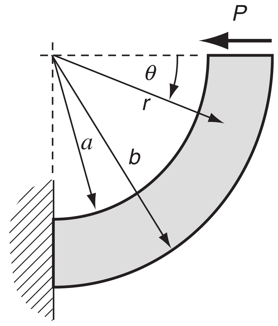
The curved cantilever beam is fixed on the left side, and the right side has prescribed horizontal traction, as shown in Fig 1. The prescribed horizontal traction is \(200\) Pa. The beam's inner radius is set to \(a= 0.31\) m and the beam's outer radius to \(b = 0.33\) m. The Young's modulus is \(E= 100\) Pa and the Poisson's ratio is \(\nu = 0.3\). Gravitation effects are neglected, and there are no body forces. The problem is solved as static, using one loading increment.
Expected results
-
Stress is dependent on the angular coordinate \(\theta\);
-
The analytical solution for the stress field is [1]:
The analytical solution is generated alongside solution fields using the function object located in the system/controlDict, where one needs to input geometry and material data:
  functions
  {
      analyticalSolution
      {
          type    curvedCantileverAnalyticalSolution;

          // Inner beam radius
          rInner  0.31;

          // Outer beam radius
          rOuter  0.33;

          // Applied shear force (in N/m)
          force   4;

          // Young's modulus
          E       100;

          // Poisson's ratio
          nu      0.3;
      }
  }
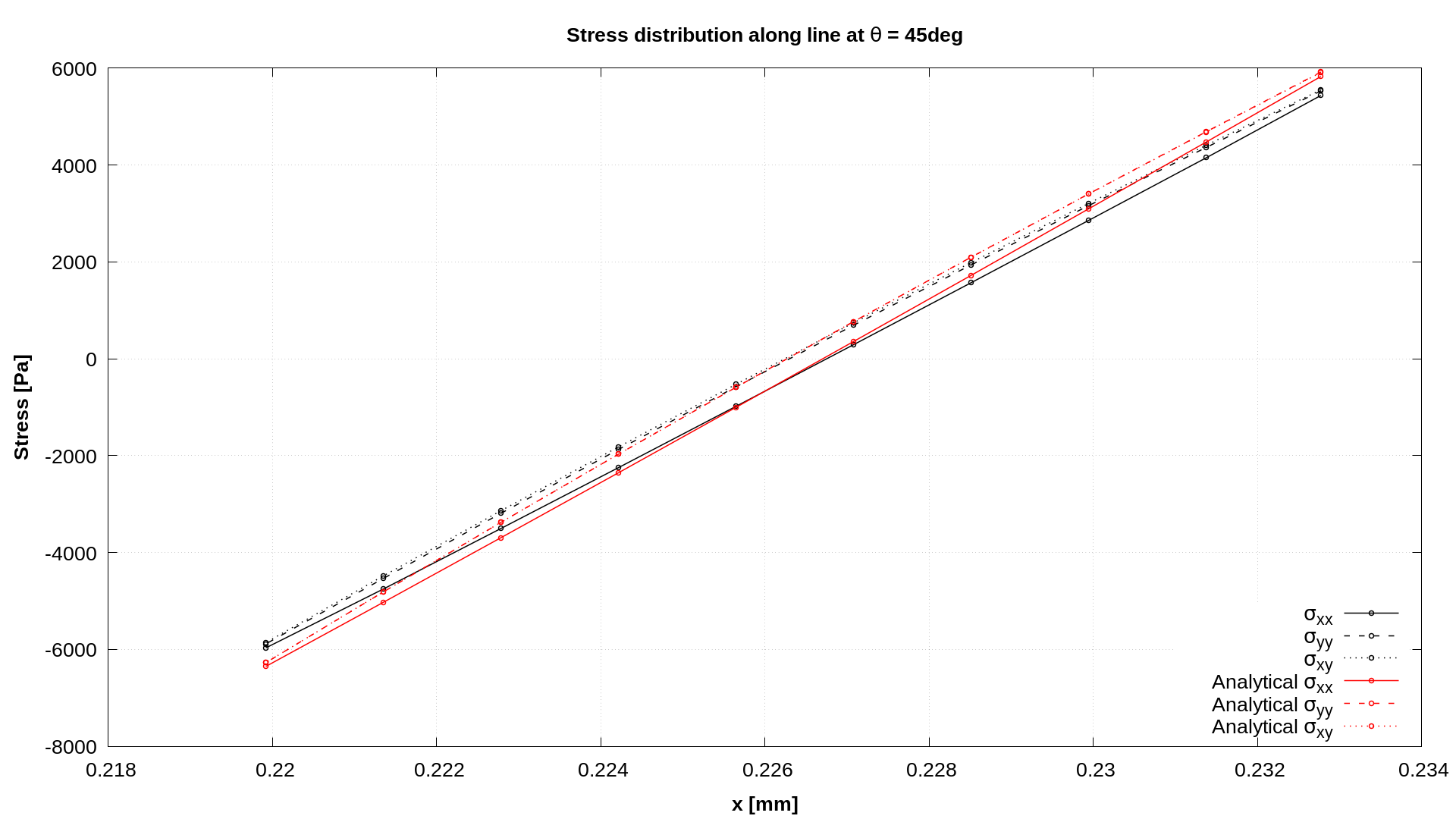
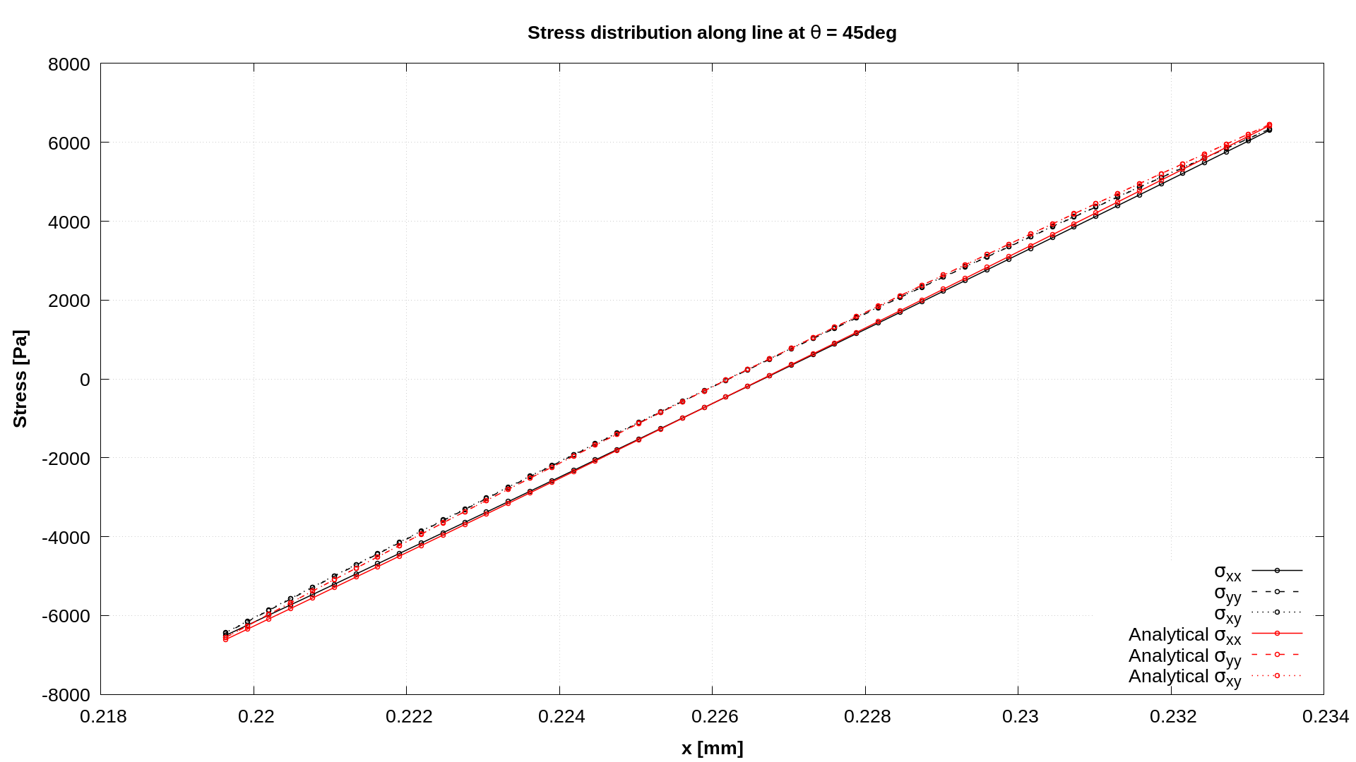
Figures 2 and 3 show \(\sigma_{xx}\), \(\sigma_{xy}\) and \(\sigma_{yy}\) stress distributions along the line \(\theta=45^{\circ}\) for computational meshes consisting of \(100\times100\) and \(200\times50\) cells. One can see that with mesh refinement, numerical results converge to analytical ones. The data for plots presented in Figures 2 and 3 is extracted using the sampleDict located in the system directory.
Running the Case
The tutorial case is located at solids4foam/tutorials/solids/linearElasticity/curvedCantilever. The case can be run using the included Allrun script, i.e. > ./Allrun. In this case, the Allrun consists of creating the mesh using blockMesh (> ./blockMesh) followed by running the solids4foam solver (> ./solids4Foam) and > ./sample utility. Optionally, if gnuplot is installed, the stress distribution is plotted in the sigmaAtTheta45deg.png file.
The coupled version of this case, which uses the coupledUnsLinearGeometryLinearElastic, can currently only be run using solids4foam built on foam-extend. To modify the case to run with the segregated linearGeometryTotalDisplacement solid model, follow the instructions in tutorials/solids/linearElasticity/narrowTmember/README.md file.
References
[1] Sadd MH. Elasticity: Theory, Applications, and Numerics. Elsevier 2009.