Solid models
Section Aims
This section aims to:
- Describe the solid models available within solids4foam;
- Provide insight into the different approaches in governing equations, linear vs nonlinear geometry, an implicit vs explicit solution algorithms.
What is a Solid Model?
In solids4foam, solid models are classes which solve the governing equations in a solid domain, primarily to calculate the deformation and related fields. These solid models (base class solidModel) can be interpretted as modular solvers, which have been packaged into a class structure. For example, one solid model may use an explicit approach to solve the governing linear momentum equation's in small strain (linear geometry) form; in contrast, another solid model may use a segregated implicit approach to solve the finite strain (nonlinear geometry) form. In general, the solid models are designed to be agnostic of the material definition; each solid model should work with any material mechanical law definition, assuming they have compatible assumptions (e.g., linear vs nonlinear geometry).
Formulating the Governing Equations
In solids4foam, most solid models take the conservation of linear momentum as the governing equation:
\[\frac{\partial (\rho \boldsymbol{v})}{\partial t} = \boldsymbol{\nabla} \cdot \boldsymbol{\sigma} + \rho \boldsymbol{b}\]Where \(\rho\) is the density, \(\boldsymbol{v}\) is the velocity vector, \(\boldsymbol{\nabla}\) is the del operator, \(\boldsymbol{\sigma}\) is the Cauchy stress tensor, and \(\boldsymbol{b}\) is a body force vector (e.g., gravity).
Vectors and tensors are represented here in bold font, while scalars are not.
A Lagrangian approach is assumed, which means that the advection/convection term disappears. One way to think of this is to consider a moving-mesh Eulerian approach (e.g. Arbitrary Eulerian-Lagrangian) where the mesh is moved at the same velocity as the underlying material; in that way, no mass enters or leaves each cell, and mass continuity is automatically satisfied.
We can equivalently express the governing equation in strong integral form:
\[\int_\Omega \frac{\partial (\rho \boldsymbol{v})}{\partial t} \; \text{d}\Omega = \oint_\Gamma \boldsymbol{n} \cdot \boldsymbol{\sigma} \; \text{d}\Gamma + \int_\Omega \rho \boldsymbol{b} \; \text{d}\Omega\]Where \(\Omega\) and \(\Gamma\) are the volume and area of the region over which we are integrating.
A key decision to be made when formulating a solution approach is to consider whether the deformations are expected to be large or not. To answer this question, consider what happens to a solid material when a force is applied: Figure 1 shows an example solid at time \(t_o\), represented by the ubiquitous continuum mechanics potato; forces are then applied to this solid and it is deformed at time \(t\). In general, a differential piece of material will change its volume from d\(\Omega_o\) to d\(\Omega\); similarly, a differential piece of the surface will change its area magnitude from d\(\Gamma_o\) to d\(\Gamma\) and its unit normal from \(\boldsymbol{n}_o\) to \(\boldsymbol{n}\). From this, it is clear that the volumes and areas in the integral form of the momentum equation are a function of the deformation field; consequently, even if the stress field is a linear function of the velocity (or displacement) field, the momentum equation will still be a nonlinear function of velocity (or displacement), as \(\Omega\) and \(\Gamma\) are a function of \(\boldsymbol{v}\).
In many practical cases, these changes in volume, area and orientation are negligible, e.g., consider how the shape of most steel structures change when loaded. In those cases, we could assume that the mesh is not a function of the material motion: this is called the linearised geometry or linear geometry assumption or, more commonly, the small strain assumption. If the changes in volume, area or orientation are not small, then no such simplifying assumption can be made, and the original nonlinear equation should be solved; this formulation is called the nonlinear geometry, finite strain, or large strain approach. Such approaches are typically required when analysing soft/flexible materials, like rubber and biological tissue, as well as in forming processes. Next, we will discuss the details of linear and nonlinear geometry approaches and their implementation in solids4foam.
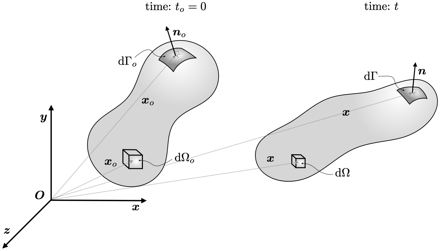
Figure 1: Deformation of a solid from the initial configuration at time \(t_o\) to the deformed configuration at time \(t\).
Linear Geometry Approach
If the change in volume, area and orientation of cells in the mesh is small, then the linear geometry assumption is valid. In that case, the linear momentum conservation can be expressed as
\[\int_{\Omega_o} \frac{\partial (\rho_o \boldsymbol{v})}{\partial t} \; \text{d}\Omega_o = \oint_{\Gamma_o} \boldsymbol{n}_o \cdot \boldsymbol{\sigma} \; \text{d}\Gamma_o + \int_{\Omega_o} \rho_o \boldsymbol{b} \; \text{d}\Omega_o\]Where subscript \(o\) indicates a quantity in the initial configuration; or, concretely, the equation is integrated over the initial mesh, which is known, and there is no need to update the mesh.
We can also derive the linear geometry formulation from an Eulerian perspective: consider momentum conservation given in Eulerian form (including the advection term); for small velocities (Reynolds numbers), the advection term can be neglected, and we arrive at the linear geometry form of the equation (similar to Stokes/creeping flow). In this way, we can see that Lagrangian and Eulerian methods coincide for linear geometry.
Nonlinear Geometry Approach
When changes in volume, area or orientation are not small, then the nonlinear geometry form of the governing equations must be solved. As the deformed position of the mesh is unknown, we must reformulate the governing equation in terms of known quantities, which are iteratively updated. Two formulations are commonly used to achieve this:
-
The total Lagrangian formulation, and
-
The updated Lagrangian formulation.
In the limit of small deformations, nonlinear geometry approaches will give the same answer as linear geometry approaches.
Total Lagrangian Formulation
The key concept behind the total Lagrangian formulation is to express the unknown mesh volumes \(\Omega\) and areas \(\boldsymbol{\Gamma}\) in terms of the known initial mesh volumes \(\Omega_o\) and areas \(\boldsymbol{\Gamma}_o\). This is achieved through Nanson's relation:
\[\boldsymbol{\Gamma} = J \boldsymbol{F}^{-T} \cdot \boldsymbol{\Gamma}_o\]Where \(\boldsymbol{F} = \textbf{I} + (\boldsymbol{\nabla}_o \boldsymbol{d})^T\) is the deformation gradient, which represents a map between material in the deformed and initial configurations; \(\textbf{I}\) is the second-order identity tensor, \(\boldsymbol{d}\) is the displacement vector, \(J = \text{det}[\boldsymbol{F}] = \frac{\Omega}{\Omega_o}\) is known as the Jacobian, and \(\boldsymbol{\nabla}_o\) makes it clear that the differential operator is performed on the initial configuration, i.e., on the initial mesh.
Using Nanson's relation and the definition of \(J\), the conservation of linear momentum can be expressed in the total Lagrangian form:
\[\int_{\Omega_o} \frac{\partial (\rho_o \boldsymbol{v})}{\partial t} \; \text{d}\Omega_o = \oint_{\Gamma_o} \left(J \boldsymbol{F}^{-T} \cdot \boldsymbol{n}_o \right) \cdot \boldsymbol{\sigma} \; \text{d}\Gamma_o + \int_{\Omega_o} \rho_o \boldsymbol{b} \; \text{d}\Omega_o\]or equivalently in differential form as
\[\frac{\partial (\rho_o \boldsymbol{v})}{\partial t} = \boldsymbol{\nabla}_o \cdot \left(J \boldsymbol{F}^{-1} \cdot \boldsymbol{\sigma} \right) \; + \rho_o \boldsymbol{b}\]As \(\boldsymbol{F}\), \(J\) and \(\boldsymbol{\sigma}\) are a function of the displacement field, the equation remains nonlinear in displacement; hence it must be iteratively solved, where \(\boldsymbol{F}\) and \(J\) are updated during the outer iterations. A convenience of the total Lagrangian approach is that the mesh is not moved; that is, the deformed configuration is calculated by integrating the governing equation over the initial mesh with appropriate mappings. If needed (e.g., for post-processing), the deformed mesh can be calculated by moving the initial mesh by the displacement field.
Updated Lagrangian Formulation
In the form given above, Nanson's relation expresses a mapping between the deformed and initial configurations; however, the expression can equivalently be given between any two configurations. Another common approach is to give Nanson's relation in terms of the deformed configuration and the configuration at the end of the last time step (the so-called updated configuration) (Figure 2):
\[\boldsymbol{\Gamma} = j \boldsymbol{f}^{-T} \cdot \boldsymbol{\Gamma}_u\]Where \(\boldsymbol{f} = \textbf{I} + (\boldsymbol{\nabla}_u \Delta \boldsymbol{d})^T\) is the relative deformation gradient, which represents a map between material in the deformed configuration and the configuration at the end of the previous time step; \(\Delta \boldsymbol{d} = \boldsymbol{d} - \boldsymbol{d}_{\text{old}}\) is the displacement increment vector, \(j = \text{det}[\boldsymbol{f}] = \frac{\Omega}{\Omega_u}\) is the relative Jacobian, and \(\boldsymbol{\nabla}_u\) is the differential operator performed on the updated configuration, i.e., on the mesh after it has been moved at the end of the previous time-step. The initial and updated configurations coincide in the first step of an analysis.
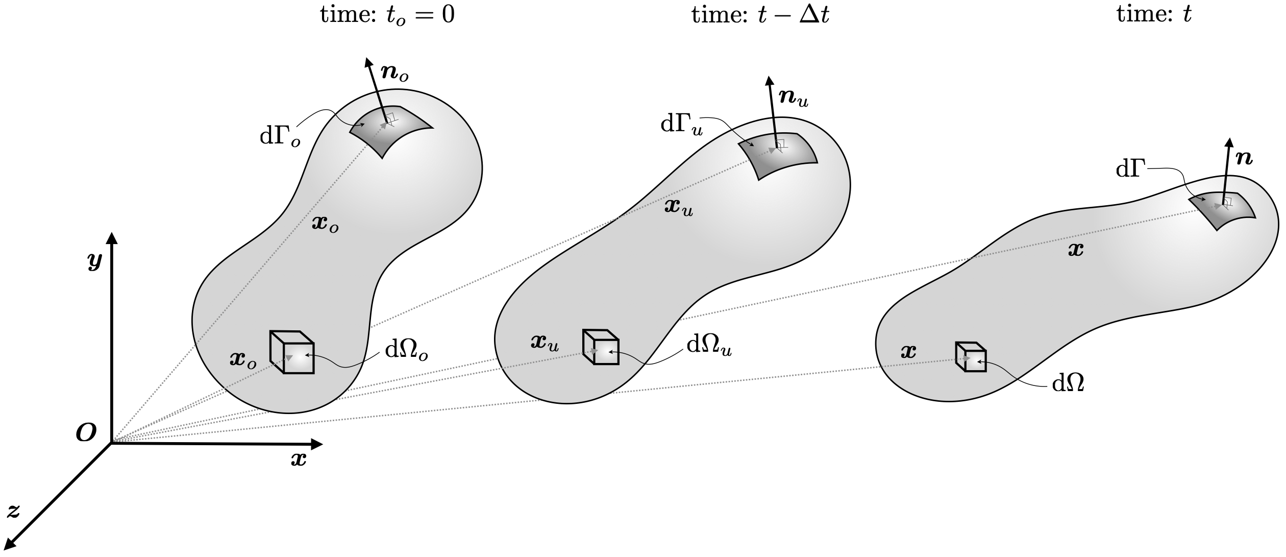
Figure 2: Deformation of a solid from the initial configuration at time \(t_o\), to the updated configuration at time \(t - \Delta t\), and finally to the deformed configuration at time \(t\).
The conservation of linear momentum can then be expressed in the updated Lagrangian form:
\[\int_{\Omega_u} \frac{\partial (\rho_u \boldsymbol{v})}{\partial t} \; \text{d}\Omega_u = \oint_{\Gamma_u} \left(j \boldsymbol{f}^{-T} \cdot \boldsymbol{n}_u \right) \cdot \boldsymbol{\sigma} \; \text{d}\Gamma_u + \int_{\Omega_u} \rho_u \boldsymbol{b} \; \text{d}\Omega_u\]or equivalently in differential form as
\[\frac{\partial (\rho_u \boldsymbol{v})}{\partial t} = \boldsymbol{\nabla}_u \cdot \left(j \boldsymbol{f}^{-1} \cdot \boldsymbol{\sigma} \right) \; + \rho_u \boldsymbol{b}\]Like the total Lagrangian approach, the updated Lagrangian approach requires an iterative solution where \(\boldsymbol{f}\) and \(j\) are updated during the outer iterations. However, unlike the total Lagrangian approach, the updated Lagrangian approach requires the mesh to be moved at the end of each time step, such that it is in the updated configuration for the subsequent step.
Solution Algorithms and Discretisations
The linear and nonlinear geometry formulations can be solved explicitly or implicitly. In explicit approaches, the \(\boldsymbol{\nabla} \cdot \boldsymbol{\sigma}\) term is calculated using the known displacement field at the previous time step. As a consequence, explicit approaches do not require the formation and solution of a linear system, but their time step size is limited by the Courant–Friedrichs–Lewy condition. In contrast, implicit approaches calculate the \(\boldsymbol{\nabla} \cdot \boldsymbol{\sigma}\) term using the unknown displacement or a combination of the unknown displacement field and the known old-time displacement field. As a result, implicit methods are unconditionally stable with no restrictions on the time step size, apart for controlling temporal accuracy.
The relative merits of explicit and implicit approaches can be summarised as:
- Explicit
- Advantages
- Each time step is fast as a linear system is not solved.
- There are no convergence problems as iteration is not required in each time step; hence, explicit methods tend to be robust at dealing with highly nonlinear problems.
- Explicit methods have excellent parallel scalability as a linear system is not solved.
- Disadvantages
- For most engineering materials, the time step size restriction can be prohibitive. Consequently, explicit methods are typically only efficient for fast problems, which occur over short time periods.
- Advantages
- Implicit
- Advantages
- The ability to use large time steps means that slow problems (i.e., static or quasi-static) can be efficiently analysed.
- Disadvantages
- For highly nonlinear problems (e.g., frictional contact, large strains, plasticity, fracture), implicit methods can struggle to converge.
- Advantages
Within solids4foam, the implicit methods can be further classified in terms of the specific solution algorithms:
-
Segregated: This is the most common approach used by solid models in solids4foam. In the segregated method, the \(\boldsymbol{\nabla} \cdot \boldsymbol{\sigma}\) term is implicitly approximated as a Laplacian term, where explicit deferred corrections ensure the original governing equation is enforced at convergence. The advantage of this approach is that it temporarily decouples the x, y and z directions of the momentum equation resulting in a memory-efficient approach. A disadvantage of this approach is that convergence of the outer iterations can be slow in quasi-static cases where the geometry has a high aspect ratio, e.g. a bending cantilever beam.
-
Coupled: The coupled or block-coupled approach aims to maximise the implicit term size by implicitly including inter-component coupling within the momentum equation. The advantage of the coupled approach is that convergence is often faster than the segregated approach for quasi-static and static problems; however, for transient problems, the segregated approach may be more competitive as the superior convergence of the coupled approach may be offset by the extra time required to form and solve the coupled system. In the special case of linear geometry, linear elasticity and linear boundary conditions, the coupled approach converges in one outer iteration, as the problem is linear.
-
Semi-Coupled: Semi-coupled approaches lie in between segregated and coupled approaches. One such approach introduces hydrostatic pressure as an additional unknown, where displacement (or velocity) and pressure are implicitly treated in a coupled manner, whereas displacement inter-component coupling in the momentum equation is still treated explicitly in a deferred correction manner. These semi-coupled approaches are similar to the coupled approaches used in fluid solvers, e.g.
pUCoupledFoamin foam-extend.
Most solid models in solids4foam are discretised using the cell-centred finite volume method; however, vertex-centred solid models are also available.
Solid Models Available in solids4foam
Here, we list the solid models currently available in soldis4foam, and brieflu summarise their characteristic features. All solid models use a cell-centred finite volume discretisation unless stated otherwise.
- Linear geometry solid models
linGeomTotalDispSolid: solves for total displacement \(\boldsymbol{d}\) (D) using a segregated approach.linGeomSolid: solves for the increment of displacement \(\Delta \boldsymbol{d}\) (DD) using a segregated approach.unsLinGeomSolid: solves for total displacement \(\boldsymbol{d}\) (D) using a segregated approach and the uns discretisation, which is more accurate but more expensive than thelinGeomTotalDispSoliddiscretisation.-
linGeomPressureDisplacementSolid: solves for total displacement \(\boldsymbol{d}\) (D) and hydrostatic pressure \(p\) (p) using a segregated PIMPLE-type algorithm. weakThermalLinGeomSolid: sequentially solves for the temperature \(T\) (T) and total displacement \(\boldsymbol{d}\) (D) in a segregated manner with no outer displacement-temperature correctors.thermalLinGeomSolid: solves for the temperature \(T\) (T) and total displacement \(\boldsymbol{d}\) (D), where outer iterations ensure convergence of the temperature-displacement coupling in a segregated manner.-
poroLinGeomSolid: solves for the pore-pressure \(p\) (p) and total displacement \(\boldsymbol{d}\) (D), where outer iterations ensure convergence of the pressure-displacement coupling in a segregated manner, based on https://doi.org/10.1002/nag.2361. coupledLinGeomPressureDisplacementSolid: similar tolinGeomPressureDisplacementSolid, except the pressure-displacement equations are solved semi-coupled; currently only available with foam-extend.coupledUnsLinGeomLinearElasticSolid: a block-coupled version ofunsLinGeomSolid, based on https://doi.org/10.1016/j.compstruc.2016.07.004; currently only available with foam-extend.-
vertexCentredLinGeomSolid: a block-coupled vertex-centred finite volume approach which solves for the total displacement at the mesh vertices/points (pointD), described in https://doi.org/10.13140/RG.2.2.22896.33283; this solver currently works best with triangular and tetrahedral grids. explicitLinGeomTotalDispSolid: an explicit version oflinGeomTotalDispSolid.-
explicitUnsLinGeomTotalDispSolid: an explicit version ofunsLinGeomSolid. kirchhoffPlateSolid: this model solves the Kirchhoff plate equations using a segregated finite area method; currently only available with foam-extend.
- Nonlinear geometry solid models
nonLinGeomTotalLagTotalDispSolid: a total Lagrangian nonlinear geometry version oflinGeomTotalDispSolid.nonLinGeomTotalLagSolid: a total Lagrangian nonlinear geometry version oflinGeomSolid.nonLinGeomUpdatedLagSolid: an updated Lagrangian nonlinear geometry version oflinGeomSolid.unsNonLinGeomTotalLagSolid: a total Lagrangian nonlinear geometry version ofunsLinGeomSolid.unsNonLinGeomUpdatedLagSolid: an updated Lagrangian nonlinear geometry version ofunsLinGeomSolid, except that the primary solution variable is the increment of displacement \(\Delta \boldsymbol{d}\) (DD).coupledNonLinGeomPressureDisplacementSolid: a total Lagrangian nonlinear geometry version ofcoupledLinGeomPressureDisplacementSolid; currently only available with foam-extend.