Indentation of elastic half-space with a flat-ended rigid indenter: flatEndedRigidIndenter
Prepared by Ivan Batistić
Tutorial Aims
- Demonstrate the analysis of a contact problem between rigid and deformable bodies.
- Determine the accuracy of the solver for a contact problem by comparing its predictions with an available analytical solution.
Case Overview
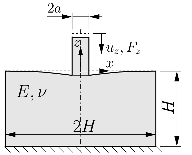
This case consists of a rigid flat-ended indenter pressed onto an elastic-half space (Figure 1). The elastic half-space is modelled as finite, with dimensions \(2H \times H\), a Young's modulus \(E = 200\) GPa and a Poisson's ratio \(\nu= 0.3\). The problem is solved by assuming a plane stress state and a 2-D model with unit thickness. The top surface of the rigid indenter has a prescribed vertical displacement \(u_z = 0.0967\) mm corresponding to vertical force \(F_z = 10 000\) N (see Eq (4)). The bottom surface of the finite half-space is held fixed (zero displacement). The contact between the punch and the elastic half-space is modelled as frictionless.
Expected Results
The analytical solution for the pressure distribution (plane stress) is [2]:
\[p_n(x) = \frac{F}{\pi\sqrt{a^2-x^2}} \qquad \text{for } |x| \leq a,\]where \(a\) is half the contact width and \(x\) is the horizontal coordinate. This pressure distribution is singular at the edge (\(x \equiv \pm a\)) of the fixed contact zone.
The displacement of the rigid indentor \(d\), related to the applied force \(F\), can be obtained using:
\[u_z = \frac{F}{\pi E}\left[ 2 \text{ln} \left(\frac{2L}{a}\right) - (1+\nu) \right],\]where \(L\) is the thickness of the elastic half-space.
The boundary displacement outside the contact zone can be calculated as:
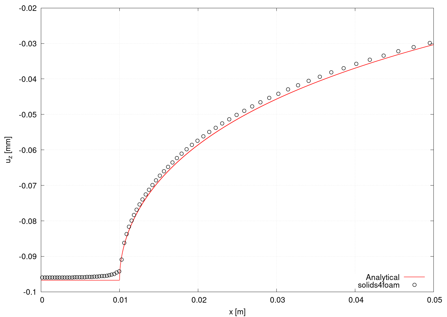
\[u_z(x) = u_z + \frac{2(1-\nu^2)F}{\pi E} \text{ ln} \left[ \frac{x}{a} + \sqrt{\frac{x^2}{a^2}-1} \right] \qquad \text{for } |x| \geq a.\]Figure 2 shows the distribution of the contact pressure. The diagram is created automatically within the Allrun script using sample utility and gnuplot. Further mesh refinement would lead to a closer approximation of the analytical solution. As the mesh is refined, the predicted contact pressure at the contact edge goes to infinity, as expected.
The main cause of the shift between the analytical and the numerical curve is the applied pressure calculation method in the solidContact boundary condition. The arising error can be reduced with mesh refinement or by using the pressure integration method proposed in [1] (this improved contact condition will soon be available in solids4foam).
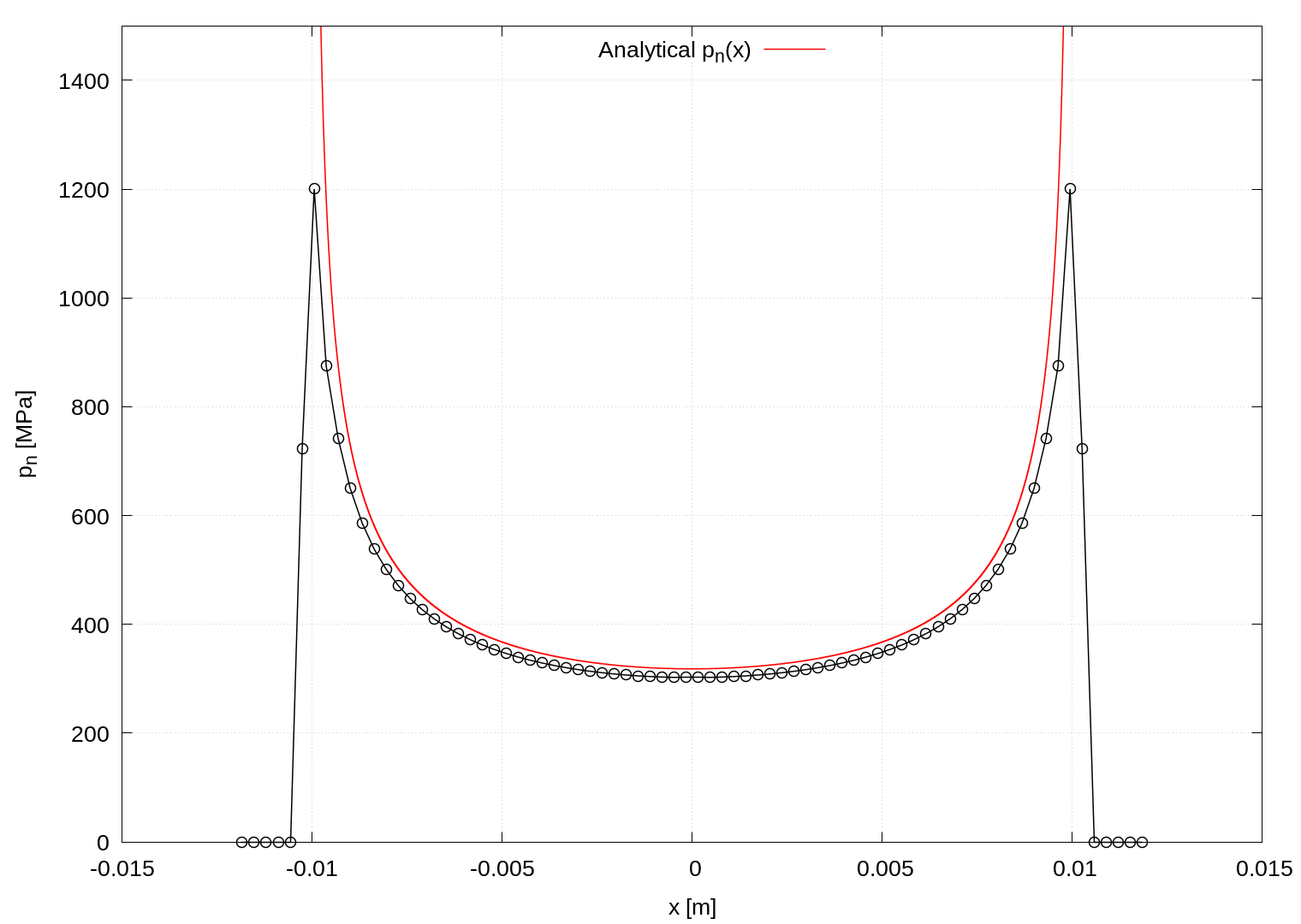
Figure 3 shows the displacement profile of the half-space top surface. The displacement profile from solids4Foam matches the analytical one; a small discrepancy between results exists because the analytical solution has an abrupt profile change at the contact edge. As in Figure 2, the diagram shown in Figure 3 is automatically created within the Allrun script using sample utility and gnuplot.
Running the Case
The tutorial case is located at solids4foam/tutorials/solids/linearElasticity/flatEndedRigidIndenter. The case can be run using the included Allrun script, i.e. > ./Allrun. In this case, the Allrun consists of creating the mesh using blockMesh (> blockMesh) followed by running the solids4foam solver (> solids4Foam). Optionally, if gnuplot is installed, the stress distribution is plotted in the pressureDistribution.png file.
References
[2] K. L. Johnson, Contact Mechanics. Cambridge University Press, 1985.